Fitting a Linear ACE Potential
This notebook picks up where SimpleUnary leaves off: it reads the
training dataset produced there and fits a simple linear pair-descriptor ACE
potential with python-ace.
Prerequisites
Run SimpleUnary first so that Unary/2/everything_training_data.pckl.gz
exists. Then install the optional python-ace package:
pip install python-ace
What this notebook covers
Load the training dataframe from SimpleUnary.
Define a minimal linear ACE basis (pair descriptors only).
Fit the potential with ridge regression via
LinearACEFit.Evaluate train errors (MAE / RMSE on energies and forces).
Inspect the resulting pair potential against the Morse reference.
Imports
import numpy as np
import pandas as pd
import matplotlib.pyplot as plt

import pyace
import pyace.linearacefit as plf
from ase import Atoms
from ase.calculators.morse import MorsePotential
/home/ponder/micromamba/envs/assyst/lib/python3.12/site-packages/pyace/multispecies_basisextension.py:4: UserWarning: pkg_resources is deprecated as an API. See https://setuptools.pypa.io/en/latest/pkg_resources.html. The pkg_resources package is slated for removal as early as 2025-11-30. Refrain from using this package or pin to Setuptools<81.
  import pkg_resources
Load training data
The dataframe was saved by SimpleUnary and contains one row per structure
with columns ase_atoms, energy (eV), forces (eV/Å), and number_of_atoms.
max_num = 2  # match the value used in SimpleUnary

df = pd.read_pickle(f'Unary/{max_num}/everything_training_data.pckl.gz')
print(f"Loaded {len(df)} structures")
df.head()
Loaded 1573 structures
| ase_atoms | energy | forces | number_of_atoms | |
|---|---|---|---|---|
| 0 | (Atom('Cu', [-1.3265240321355765, -7.353189190... | -1.802887 | [[6.071532165918825e-18, -7.979727989493313e-1... | 1 |
| 1 | (Atom('Cu', [0.0, 0.0, 0.24375080364530244], i... | -2.192044 | [[7.556889142223966e-17, 2.886146183156413e-16... | 1 |
| 2 | (Atom('Cu', [0.0, 0.0, 0.0], index=0)) | -1.702372 | [[4.5102810375396984e-17, 1.708702623837155e-1... | 1 |
| 3 | (Atom('Cu', [-1.1459510315187336, -1.145951031... | -1.921211 | [[6.895525817007808e-17, -3.673276960380889e-1... | 1 |
| 4 | (Atom('Cu', [-0.7029469904758565, 1.2175399025... | -2.453490 | [[5.204170427930421e-18, 7.28583859910259e-17,... | 1 |
Define the ACE basis
We use the simplest possible ACE expansion: a linear, pair-descriptor-only
potential (order 1, lmax=0) with moderate basis size and cut off.
def make_ace_basis(rmax, number_of_radial_functions, element='Cu'):
    """Minimal linear pair-descriptor ACE basis for a single element."""
    pot_conf = {
        'elements': [element],
        'embeddings': {
            'ALL': {
                'fs_parameters': [1, 1],
                'ndensity': 1,
                'npot': 'FinnisSinclair',
            },
        },
        'bonds': {
            'ALL': {
                'NameOfCutoffFunction': 'cos',
                'dcut': 0.01,
                'radbase': 'ChebPow',
                'radparameters': [2.0],
                'rcut': rmax,
            },
        },
        'functions': {
            'UNARY': {
                'nradmax_by_orders': [number_of_radial_functions],
                'lmax_by_orders':    [0],
            }
        }
    }
    return pyace.create_multispecies_basis_config(pot_conf)


bbasis = make_ace_basis(rmax=6.5, number_of_radial_functions=20, element='Cu')
Build the design matrix
LinearACEDataset projects all training structures onto the ACE basis. The
resulting design matrix has one row per energy observation plus three rows per
force component.
ds = plf.LinearACEDataset(bbasis, df)

%time ds.construct_design_matrix()
CPU times: user 6.8 ms, sys: 30.8 ms, total: 37.6 ms
Wall time: 750 ms
Fit
LinearACEFit wraps scikit-learn’s Ridge solver. For this small dataset
the fit takes milliseconds.
lf = plf.LinearACEFit(train_dataset=ds)

%time lf.fit()
CPU times: user 3.54 ms, sys: 940 μs, total: 4.48 ms
Wall time: 5.14 ms
Ridge(alpha=1e-05, copy_X=False, fit_intercept=False, random_state=42)In a Jupyter environment, please rerun this cell to show the HTML representation or trust the notebook.
On GitHub, the HTML representation is unable to render, please try loading this page with nbviewer.org.
Parameters
| alpha | 1e-05 | |
| fit_intercept | False | |
| copy_X | False | |
| max_iter | None | |
| tol | 0.0001 | |
| solver | 'auto' | |
| positive | False | |
| random_state | 42 |
Training errors
compute_errors returns MAE and RMSE for energies per atom (epa_*) and
force components (f_comp_*).
lf.compute_errors()
{'epa_mae': 0.002855277384345856,
 'epa_rmse': 0.0037819909234652733,
 'f_comp_mae': 0.0016788159377372038,
 'f_comp_rmse': 0.003674505978445838}
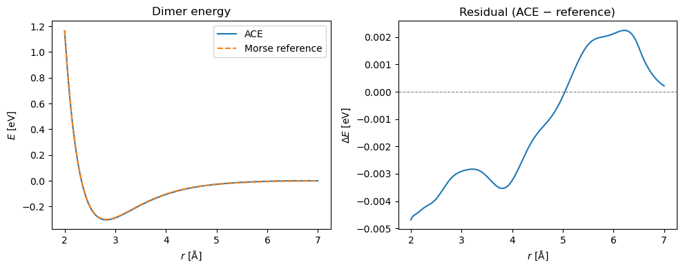
Inspect the fitted pair potential
A dimer curve (two Cu atoms at varying separation) is an easy sanity check: the ACE potential should reproduce the Morse reference minimum near 2.8 Å.
def dimer_curve(calc, r_values):
    """Evaluate a dimer energy curve for a given ASE calculator.

    Args:
        calc: ASE calculator
        r_values: 1-D array of Cu–Cu distances in Å

    Returns:
        (r_values, energies) — both as numpy arrays
    """
    energies = []
    for r in r_values:
        s = Atoms(['Cu', 'Cu'], positions=[[0, 0, 0], [r, 0, 0]], cell=[40] * 3)
        s.calc = calc
        energies.append(s.get_potential_energy())
    return r_values, np.array(energies)


acef      = pyace.PyACECalculator(lf.get_bbasis())
reference = MorsePotential(epsilon=0.3, r0=2.55265548 * 1.10619396, rho0=4)

r = np.linspace(2.0, 7.0, 200)
_, e_ace = dimer_curve(acef, r)
_, e_ref = dimer_curve(reference, r)

fig, (ax1, ax2) = plt.subplots(1, 2, figsize=(10, 4))

ax1.plot(r, e_ace, label='ACE')
ax1.plot(r, e_ref, label='Morse reference', linestyle='--')
ax1.set_xlabel(r'$r$ [Å]')
ax1.set_ylabel(r'$E$ [eV]')
ax1.legend()
ax1.set_title('Dimer energy')

ax2.plot(r, e_ace - e_ref)
ax2.axhline(0, color='gray', linewidth=0.8, linestyle='--')
ax2.set_xlabel(r'$r$ [Å]')
ax2.set_ylabel(r'$\Delta E$ [eV]')
ax2.set_title('Residual (ACE − reference)')

plt.tight_layout()