A Complete Workflow for a Single Element

This notebook runs the full ASSYST pipeline end-to-end on a unary system (copper). The four canonical steps are:

1. Sampling — generate symmetric random structures for every space group.

2. Relaxing — minimise volume first, then full cell + positions, to find the relevant pockets of the potential energy surface.

3. Perturbing — apply random rattles and stretches around those minima to populate the surrounding PES.

4. Combining — collect everything, filter unphysical configurations, evaluate the reference and store the resulting training data.

In a real workflow the relaxations and final evaluations are carried out with DFT (or any other reference); here we use a Morse potential so the notebook runs quickly.

Imports

import pickle
from pathlib import Path

import numpy as np
import pandas as pd
import matplotlib.pyplot as plt
from tqdm.auto import tqdm

from assyst.crystals import Formulas, sample
from assyst.filters import DistanceFilter, AspectFilter, VolumeFilter
from assyst.relaxations import VolumeRelax, FullRelax, relax
from assyst.perturbations import RandomChoice, Rattle, Stretch, perturb

Configuration

max_num is the largest number of atoms per generated structure. 2 keeps the example fast; 10 is the typical production value and yields ~10k training structures.

max_num = 2
out_dir = Path(f"Unary/{max_num}")
out_dir.mkdir(parents=True, exist_ok=True)

Reference potential

Any ASE calculator works. We pick a Morse potential whose parameters were chosen so that its minimum sits near the experimental Cu-Cu bond length.

For more interesting reference data the universal Grace graph-ACE models in assyst.calculators are a good drop-in replacement (they require the optional tensorpotential dependency).

from ase.calculators.morse import MorsePotential

reference = MorsePotential(epsilon=0.3, r0=2.55265548 * 1.10619396, rho0=4)

1. Sampling random structures

Build the formulas to sample (Cu, Cu_2, …, up to max_num) and let sample generate one structure for every compatible space group.

AspectFilter(6) filters out very elongated unit cells that pyxtal occasionally produces.

formulas = Formulas.range('Cu', max_num + 1)
formulas

Formulas(atoms=({'Cu': 0}, {'Cu': 1}, {'Cu': 2}))

spg = list(filter(
    AspectFilter(6),
    sample(
        formulas,
        spacegroups=range(1, 230 + 1),
        max_atoms=max_num,
    )
))
print(f"Generated {len(spg)} symmetric seeds")

Generated 167 symmetric seeds

Each entry is an :class:ase.Atoms carrying the sampled cell and positions. A small summary of the first few sampled structures:

pd.DataFrame([
    {
        'formula': s.get_chemical_formula(),
        'natoms': len(s),
        'volume_per_atom': s.cell.volume / len(s),
    }
    for s in spg[:5]
])

	formula	natoms	volume_per_atom
0	Cu	1	10.911529
1	Cu	1	11.704551
2	Cu	1	11.899922
3	Cu	1	12.247109
4	Cu	1	11.184826

Just to create a small check point, dump generated structures into a pickle file. This is not required for assyst.

with open(out_dir / 'spg.pckl', 'wb') as f:
    pickle.dump(spg, f)

2. Relaxation

ASSYST applies a two-step relaxation:

1. VolumeRelax — relax the volume only, keeping shape and internal positions frozen. Quickly puts each seed near a sensible energy scale.

2. FullRelax — relax cell shape, volume and atomic positions together, landing in a (local) minimum of the PES.

In production both would be carried out with DFT; here the Morse potential makes the cost negligible. For experimentation, assyst.relaxations also provides CellRelax and SymmetryRelax.

volset = VolumeRelax(max_steps=100, force_tolerance=1e-3)
allset = FullRelax(max_steps=100, force_tolerance=1e-3)

%%time
volmin = list(relax(tqdm(spg, desc='volume'), volset, reference))

CPU times: user 1min 2s, sys: 55.4 ms, total: 1min 2s
Wall time: 21 s

%%time
allmin = list(relax(tqdm(volmin, desc='full'), allset, reference))

CPU times: user 4min, sys: 414 ms, total: 4min
Wall time: 1min 25s

relax returns a new list of :class:ase.Atoms. Comparing the volume per atom before and after each relaxation step shows how the cells shrink towards their minima:

pd.DataFrame({
    'sampled':  [s.cell.volume / len(s) for s in spg[:5]],
    'volmin':   [s.cell.volume / len(s) for s in volmin[:5]],
    'allmin':   [s.cell.volume / len(s) for s in allmin[:5]],
})

	sampled	volmin	allmin
0	10.911529	15.667167	11.761170
1	11.704551	13.639392	11.761452
2	11.899922	44.776388	12.829227
3	12.247109	13.261506	12.829213
4	11.184826	54.634555	298.602200

with open(out_dir / 'volmin.pckl', 'wb') as f:
    pickle.dump(volmin, f)
with open(out_dir / 'allmin.pckl', 'wb') as f:
    pickle.dump(allmin, f)

3. Random perturbations

Around each minimum we sample the surrounding PES with three families of random perturbations described in the ASSYST paper:

1. mostly positional noise with a small cell change (rattle),

2. mostly hydrostatic cell change,

3. mostly shear cell change.

The hydrostatic and shear strains are combined with RandomChoice so that hydrostatic changes are drawn slightly more often. The final mods sequence is applied to every fully-minimised structure. DistanceFilter discards perturbations that placed atoms unphysically close.

rattle = Rattle(0.25) + Stretch(hydro=0.05, shear=0.005)
hydro = Stretch(hydro=0.80, shear=0.05)
shear = Stretch(hydro=0.05, shear=0.20)
stretch = RandomChoice(hydro, shear, 0.7)

# four rattles + four stretches per minimum reproduces the published settings
mods = 4 * [rattle] + 4 * [stretch]

%%time
random = list(perturb(allmin, mods, filters=[DistanceFilter({'Cu': 1})]))
print(f"Produced {len(random)} perturbed structures")

Produced 1188 perturbed structures
CPU times: user 497 ms, sys: 6.98 ms, total: 504 ms
Wall time: 429 ms

Each relaxed minimum is expanded into a cloud of perturbed structures. Looking at the spread of volumes per atom around the first minimum gives a feel for the noise applied:

ref = allmin[-1]
v0 = ref.cell.volume / len(ref)
siblings = [s for s in random if s.info['seed'] == ref.info['seed']]
pd.DataFrame([
    {
        'natoms': len(s),
        'volume_per_atom': s.cell.volume / len(s),
        'rel_volume_change': s.cell.volume / len(s) / v0 - 1,
    }
    for s in siblings
])

	natoms	volume_per_atom	rel_volume_change
0	2	11.764033	0.000484
1	2	11.468011	-0.024692
2	2	11.943824	0.015774
3	2	10.899526	-0.073039
4	2	11.717989	-0.003432
5	2	11.878374	0.010208
6	2	11.415293	-0.029175
7	2	11.321541	-0.037148

with open(out_dir / 'random.pckl', 'wb') as f:
    pickle.dump(random, f)

4. Combine and evaluate

Concatenate the sampled, relaxed and perturbed structures, run the distance and volume filters once more to reject any leftover pathological configurations, and finally evaluate the reference to obtain a training dataset of energies and forces.

everything = list(filter(
    VolumeFilter(300),
    filter(DistanceFilter({'Cu': 1}), spg + volmin + allmin + random),
))
print(f"Final training set: {len(everything)} structures")

Final training set: 1565 structures

rows = []
for s in tqdm(everything, desc='evaluating'):
    s.calc = reference
    rows.append({
        'ase_atoms': s,
        'energy': s.get_potential_energy(),
        'forces': s.get_forces(),
        'number_of_atoms': len(s),
    })
df = pd.DataFrame(rows)
df.to_pickle(out_dir / 'everything_training_data.pckl.gz')
df.head()

	ase_atoms	energy	forces	number_of_atoms
0	(Atom('Cu', [-1.0386276484191481, -0.194573218...	-2.168733	[[3.191891195797325e-16, -2.8622937353617317e-...	1
1	(Atom('Cu', [0.6736784829368637, -1.1197747671...	-2.354713	[[-7.592633932598097e-17, 6.227072826023132e-1...	1
2	(Atom('Cu', [0.0, -1.1901120180848723, -7.2873...	-1.787319	[[4.0722633598555547e-16, -8.066464163292153e-...	1
3	(Atom('Cu', [0.0, 0.0, -1.3521411060002535], i...	-1.345679	[[-2.0643209364124004e-16, -5.204170427930421e...	1
4	(Atom('Cu', [-1.0311953554480588, -1.031195355...	-1.358783	[[-3.226585665316861e-16, -2.42861286636753e-1...	1

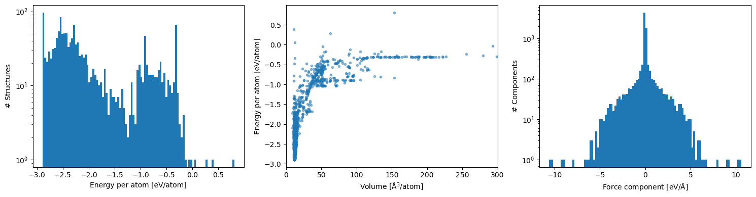
Inspect the training data

Energy per atom, energy vs volume and force component distributions are a quick sanity check that the dataset spans the expected ranges.

fig, axes = plt.subplots(1, 3, figsize=(15, 4))

(df['energy'] / df['number_of_atoms']).plot.hist(bins=100, log=True, ax=axes[0])
axes[0].set_xlabel('Energy per atom [eV/atom]')
axes[0].set_ylabel('# Structures')

axes[1].scatter(
    df['ase_atoms'].map(lambda s: s.cell.volume / len(s)),
    df['energy'] / df['number_of_atoms'],
    marker='.', alpha=0.5,
)
axes[1].set_xlim(0, 300)
axes[1].set_xlabel(r'Volume [$\mathrm{\AA}^3$/atom]')
axes[1].set_ylabel('Energy per atom [eV/atom]')

df['forces'].explode().explode().infer_objects().plot.hist(bins=100, log=True, ax=axes[2])
axes[2].set_xlabel(r'Force component [eV/$\mathrm{\AA}$]')
axes[2].set_ylabel('# Components')

plt.tight_layout()

Optional: post-hoc filtering

If the resulting energies and forces still cover ranges that are too extreme, EnergyFilter and ForceFilter (or pandas query) can prune them. These act on ase.Atoms objects that carry a SinglePointCalculator, which is what relax and the loop above attach.

df.query('-3 <= energy / number_of_atoms < 10')

	ase_atoms	energy	forces	number_of_atoms
0	(Atom('Cu', [-1.0386276484191481, -0.194573218...	-2.168733	[[3.191891195797325e-16, -2.8622937353617317e-...	1
1	(Atom('Cu', [0.6736784829368637, -1.1197747671...	-2.354713	[[-7.592633932598097e-17, 6.227072826023132e-1...	1
2	(Atom('Cu', [0.0, -1.1901120180848723, -7.2873...	-1.787319	[[4.0722633598555547e-16, -8.066464163292153e-...	1
3	(Atom('Cu', [0.0, 0.0, -1.3521411060002535], i...	-1.345679	[[-2.0643209364124004e-16, -5.204170427930421e...	1
4	(Atom('Cu', [-1.0311953554480588, -1.031195355...	-1.358783	[[-3.226585665316861e-16, -2.42861286636753e-1...	1
...	...	...	...	...
1560	(Atom('Cu', [0.1381167850060396, -0.1182780644...	-4.905344	[[-3.971783227794896, 1.8061865367255856, 1.07...	2
1561	(Atom('Cu', [0.0, 0.0, 0.0], index=0), Atom('C...	-4.404489	[[-1.345494896054511e-15, -7.971054372113429e-...	2
1562	(Atom('Cu', [0.0, 0.0, 0.0], index=0), Atom('C...	-4.565983	[[-5.88938620094126e-16, -6.934557095217286e-1...	2
1563	(Atom('Cu', [0.0, 0.0, 0.0], index=0), Atom('C...	-4.377709	[[-4.077282877100984e-15, 5.11729872886002e-16...	2
1564	(Atom('Cu', [0.0, 0.0, 0.0], index=0), Atom('C...	-5.381921	[[3.2067447655603765e-15, 2.912600716165059e-1...	2

1565 rows × 4 columns

Next steps

This notebook stops at the training set. Fitting a potential is then the job of a downstream MLIP package — e.g. ACE via python-ace, MTP via mlip-3, or any other framework that reads a list of structures with energies and forces. The dataframe saved in Unary/<max_num>/everything_training_data.pckl.gz is in the format consumed by pyace.linearacefit.LinearACEDataset.

The companion notebook ACEFitting.ipynb walks through training a small linear ACE potential on the dataset produced here.